We'll ignore any backlighting for now and reverse the parameterization through the volume so that $t$ is the parameter at the back of the volume (where photons enter) and 0 is the parameter at the front of the volume (where photons exit). Then $$I(0) = \int_0^t C(s)\ \tau(s)\ ds\ e^{-\int_0^s \tau(u)\ du}$$
Step 1: Discretize the integral
To evaluate this, we will first approximate the integral with a sum. In other words, $$\int ds \rightarrow \sum \Delta s$$
for finite intervals of size $\Delta s$:
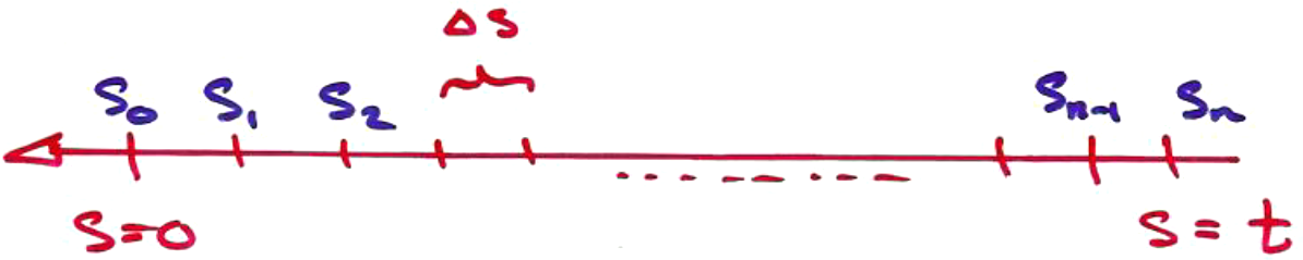
Above, we have $$s_i = i\ \Delta s$$ $$\Delta s = {t \over n} \qquad \textrm{for } n \textrm{ intervals}$$
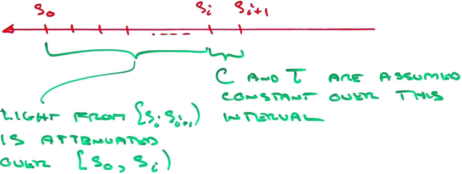
Assume that the colour, $C$, and the absorption, $\tau$, are constant over the interval $[ s_i, s_{i+1} )$: $$C_i = C(s_i)$$ $$\tau_i = \tau(s_i)$$
Step 2: Approximate the attenuation
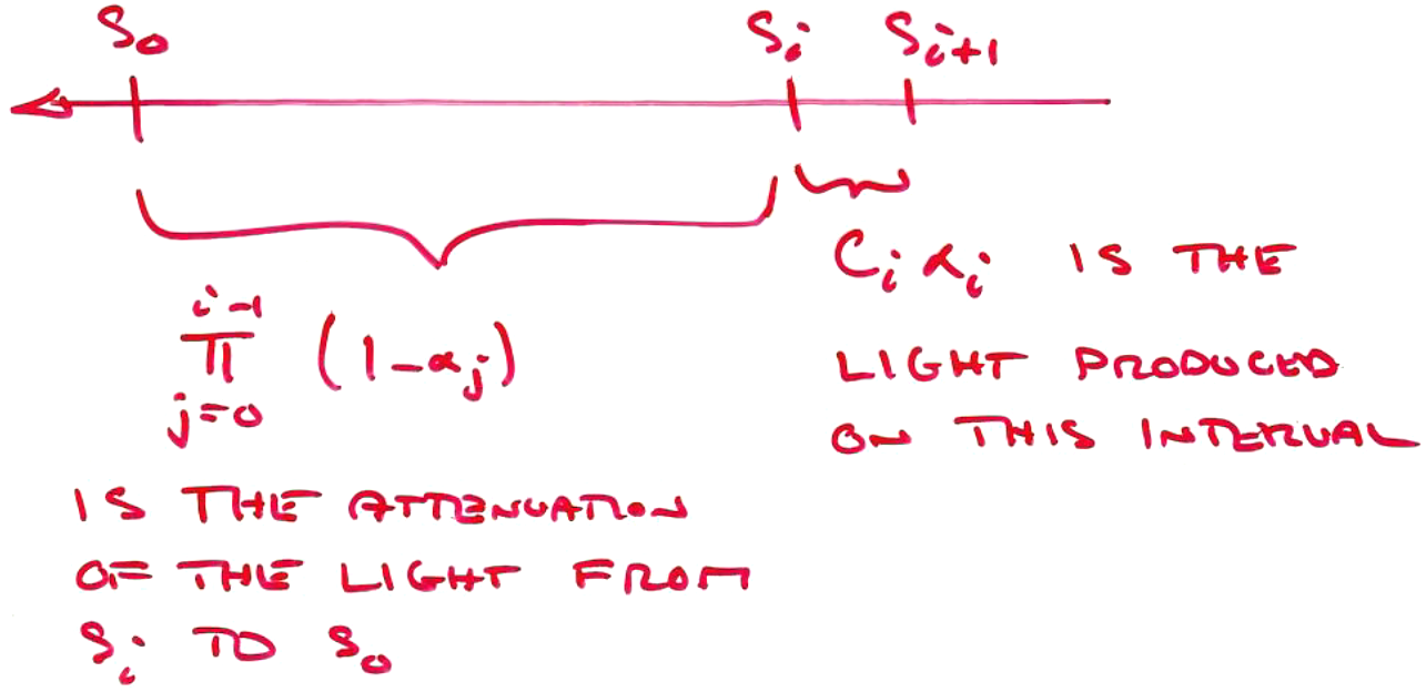
The attenuation from $s_i$ to $s_0$ is $$e^{-\int_{s_0}^{s_i} \tau(u)\ du}$$
which can be split into intervals $$e^{-\int_{s_0}^{s_i} \tau(u)\ du} = e^{-\int_{s_0}^{s_1} \tau(u)\ du} \times e^{-\int_{s_1}^{s_2} \tau(u)\ du} \times \ldots \times e^{-\int_{s_{i-1}}^{s_i} \tau(u)\ du}$$
(since $a^{\int_b^c \cdots + \int_c^d \cdots} = a^{\int_b^c \cdots} \times a^{\int_c^d \cdots}$).
We've assumed that $\tau(u) = \tau_i$ over $[ s_i, s_{i+1})$, so $$\begin{array}{rcl} e^{-\int_{s_j}^{s_{j+1}} \tau(u)\ du} &=& e^{-\int_{s_j}^{s_{j+1}} \tau_j\ du} \\ &=& e^{-\tau_j\ \int_{s_j}^{s_{j+1}}\ du} \\ &=& e^{-\tau_j\ \Delta s} \end{array}$$
Then the approximation (due to our assumption of a constant $\tau_i$) is $$\begin{array}{rcl} e^{-\int_{s_0}^{s_i} \tau(u)\ du} &\approx& e^{-\tau_0\ \Delta s} \times e^{-\tau_1\ \Delta s} \times e^{-\tau_2\ \Delta s} \times \ldots \times e^{-\tau_{i-1}\ \Delta s} \\ &=& \displaystyle \prod_{j=0}^{i-1} e^{-\tau_j\ \Delta s} \end{array}$$
Step 3: Write in terms of opacity
Define the opacity as $$\begin{array}{rcl} \alpha_j &=& \tau_j\ \Delta s \\ &=& { \mathrm{density} \over \mathrm{distance} } \times \small\mathrm{distance} \end{array}$$
Then $$e^{-\tau_j\ \Delta s} = e^{-\alpha_j}$$
Step 4: Further approximate with a Taylor series
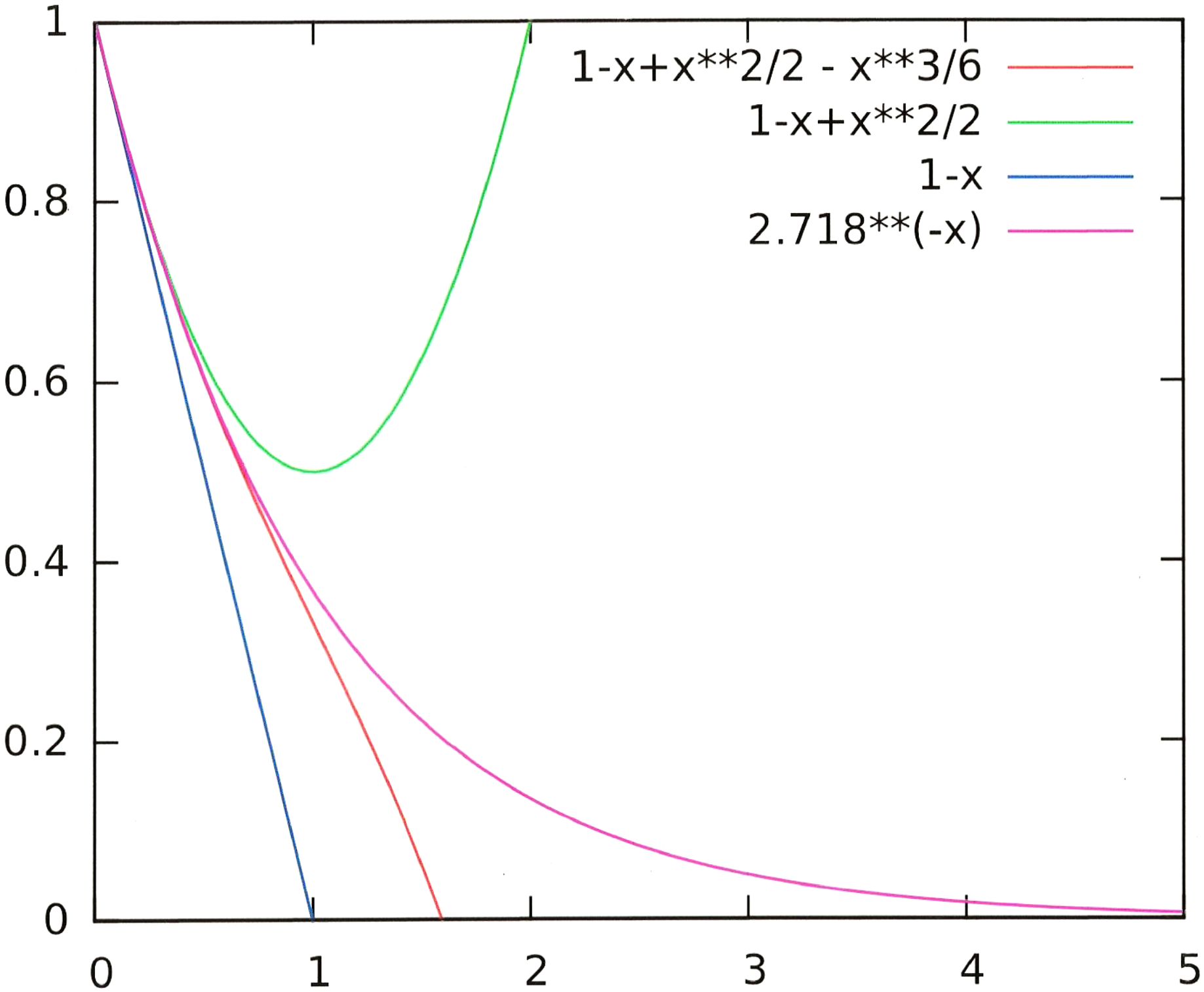
Recall the Taylor expansion of $e^k$: $$\begin{array}{rcl} e^{-\alpha} &=& 1 + {-\alpha \over 1} + {(-\alpha)^2 \over 2!} + {(-\alpha)^3 \over 3!} + \cdots \\ &=& 1 - \alpha + \underbrace{{\cal O}( \alpha^2 )}_{\textrm{small compared to } \alpha} \\ &\approx& 1 - \alpha \end{array}$$
We're approximating $e^{-\alpha}$ in purple below with $1-\alpha$ in blue below. As long as $\alpha$ is small, this works. (The green curve is three terms of the Taylor series, while the orange curve is four terms. We could get more accuracy by adding another term, but this is almost never done.)
Step 5: Build the Discrete Volume Rendering Integral
Putting everything together: $$\begin{array}{rcl} L &=& \displaystyle \int_0^t C(s)\ \tau(s)\ e^{-\int_0^s \tau(u)\ du}\ ds \\ L &\approx& \displaystyle \sum_{i=0}^n C_i\ \tau_i\ \Delta s\ \left(\ \prod_{j=0}^{i-1}\ e^{-\tau_j\ \Delta s}\ \right) \\ L &\approx& \displaystyle \sum_{i=0}^n C_i\ \alpha_i\ \left(\ \prod_{j=0}^{i-1}\ (1-\alpha_j)\ \right) \end{array}$$
This diagram may give some intuition:
Step 6: Add Backlighting
The discrete VRI has a term in which $i = n$. There is no interval $[n,n+1)$, so we will use this last term to add backlighting, in the case of DRR rendering.
Then the discrete VRI is $$\Lout = \displaystyle \sum_{i=0}^n C_i\ \alpha_i\ \left(\ \prod_{j=0}^{i-1}\ (1-\alpha_j)\ \right)$$
where we define $$C_n\ \alpha_n = \Lin$$
as the backlighting. Note that this $\Lin$ gets correctly attenuated across the whole volume by the term $\prod_{j=0}^{n-1}\ (1-\alpha_j)$.