"MIP" is from the Latin "multum in parvo", meaning "much in little".
The problem addressed with mip-maps is that many texels might project to the same pixel, so a pixel should be coloured by the average colour of the texels that project to it.

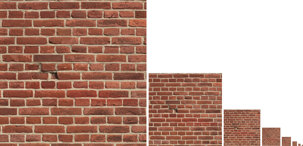
A mip-map consists of a $2^k \times 2^k$ base texture map, plus a set of reduced texture maps of sizes
$2^{k-1} \times 2^{k-1}, \; \; 2^{k-2} \times 2^{k-2}, \; \; \ldots \; \; 4 \times 4, \; \; 2 \times 2, \; \; 1 \times 1$
Each pixel in the $2^{i-1} \times 2^{i-1}$ map is the average colour of four pixels (a $2 \times 2$ block) in the larger $2^i \times 2^i$ map.

The averaging of texels is noticable in the smaller (coarser) levels:
Which Level to Use?
When looking up a texture value, the texture unit picks the mip-map level at which a texel projects to approximately the same size as a screen pixel.
Let $T_x$ and $T_y$ be vectors on the texture map that are the projections of the $x$ and $y$ pixel edges onto the texture map, measured in unit texel dimensions. That is, if $|T_x| = 3.5$, the projection of the pixel's horizontal edge onto the texture map is 3.5 texels wide, as in the image below.
Let $p = \textrm{max}( |T_x|, |T_y| )$.
Then the mip-map level to use is $\log_2 p$, since that is the number of times $p$ has to be divided by $2$ to become the size of one texel.

How are $T_x$ and $T_y$ computed?
Let the pixel coordinates on the screen be $(x,y)$. The pixel above has coordinates $(x,y+1)$ and the pixel to the right has coordinates $(x+1,y)$.
Let $T(x,y)$ be the texture coordinates for pixel coordinates $(x,y)$. Here, $T(x,y)$ is not the texture value; it is the texture coordinates that project to pixel coordinates $(x,y)$.
Then $T_x$ is the approximately the amount that $T(x,y)$ changes as the pixel coordinate goes from $(x,y)$ to $(x+1,y)$. (This is approximate because $T_x$ may be different if measured at the top or bottom pixel edges.) In other words,
$T_x = {\large \partial T(x,y) \over \large \partial x}$
Similarly,
$T_y = {\large \partial T(x,y) \over \large \partial y}$
Recall that $T_x$ and $T_y$ are 2D vectors.
Computing the Level on the GPU
The GPU provides two functions in the fragment shader only to compute the partial derivative of a quantity with respect to the $x$ and $y$ pixel coordinates. These are dFdx( quantity ) and dFdy( quantity ).
Using those GPU functions,
$T_x$ = dFdx( texCoords )
$T_y$ = dFdy( texCoords )
So the GPU can calculate the level as
$\begin{array}{rl} \log_2 p & = \log_2( \textrm{max}( |T_x|, |T_y| ) ) \\ & = \log_2( \textrm{max}( \sqrt{ T_x \cdot T_x }, \sqrt{ T_y \cdot T_y } ) ) \\ & = \log_2( \sqrt{ \textrm{max}( \; T_x \cdot T_x, \; T_y \cdot T_y \; ) } ) \\ & = 0.5 \; \log_2( \textrm{max}( \; T_x \cdot T_x, \; T_y \cdot T_y \; ) ) \end{array}$
See getMipMapLevel in 04-textures/wavefront.frag in openGL.zip.
Trilinear Interpolation
The texture unit can also perform bilinear interpolation within a mip-map level.
Alternatively, the texture unit can pick two adjacent mip-map levels between which the screen pixel best fits. Those would be $\lfloor \log_2 p \rfloor$ and $\lfloor \log_2 p \rfloor + 1$.
Then look up the texel using bilinear interpolation in level $\lfloor \log_2 p \rfloor$, and look up the texel using bilinear interpolation in level $\lfloor \log_2 p \rfloor+1$.
Finally linearly interpolate between the two texel values in proportion to the fractional part of $\log_2 p$. This is trilinear interpolation.
See glGenerateMipmap in 04-textures/wavefront.cpp in openGL.zip.

