


The JPEG image format applies a long series of steps to compress an image. The most noticable is the division of the image into $8 \times 8$ pixel blocks, each of which is compressed independently. JPEG images use lossy compression.
At high compression levels, the division into $8 \times 8$ blocks results in a very blocky image. Shown below are two compression levels: low in the top row and high in the bottom row.
 |
 |
 |
 |
Here's an overview of how JPEG compresses an image. Details will be presented further below.
For each block:
Convert the image from RGB to YCbCr as usual.
Divide the image into $8 \times 8$ blocks. Then apply the following steps to each block, separately.
Since the eye is less sensitive to chroma variations, we can reduce the resolution of the chroma channels.
Optionally, take each $8 \times 8$ chroma block (i.e. the Cb or Cr channel) and replace it with a $4 \times 4$ block. Each of the "pixels" in a coarser block replaces a $2 \times 2$ set of pixels in the original block, and its value is the average of that set of pixels. This can also be done with a $4 \times 8$ block or an $8 \times 4$ block.
The Discrete Cosine Transform (DCT) is like the Discrete Fourier Transform (DFT), but uses a basis of cosine functions only.
There are several variants of the DCT; JPEGs use the Type-II DCT.
Applying the DCT to an $8 \times 8$ block of pixels results in an $8 \times 8$ block containing the real coefficients of the cosine basis functions, which we can then compress in Step 5.
The cosine basis functions are, for wavenumbers $u$ and $v$, $$S_{uv}(x,y) = \alpha(u)\ \alpha(v)\ \cos{ (2x+1) u \pi \over 2 \times 8 }\ \cos{ (2y+1) v \pi \over 2 \times 8 }$$
where the two 8s above come from the dimensions of the $8 \times 8$ block and $\alpha(u) = {1 \over \sqrt{2}}$ if $u =0$ and $\alpha(u) = 1$ otherwise.
Below are the 64 DCT basis functions, where white is +1, black is -1, and a mid-level grey is 0. You can see sinusoidal patterns in the top row and left column. Note that only half a period is used in these basis functions.
The 64 DCT basis functions are discrete functions that can be precomputed and stored.
To find the DCT coefficients we project the $8 \times 8$ pixel block, $f(x,y)$, onto each of the 64 basis functions, $S_{uv}(x,y)$, in turn. The coefficient for wavenumbers $u$ and $v$ is $$F(u,v) = \sum_{x=0}^7 \sum_{y=0}^7 f(x,y)\ S_{uv}(x,y)$$
The resulting coefficients can be manipulated much like we manipulated Fourier coefficients. In particular, we can suppress high frequency components by setting their coefficients to zero. More on this in Step 6.
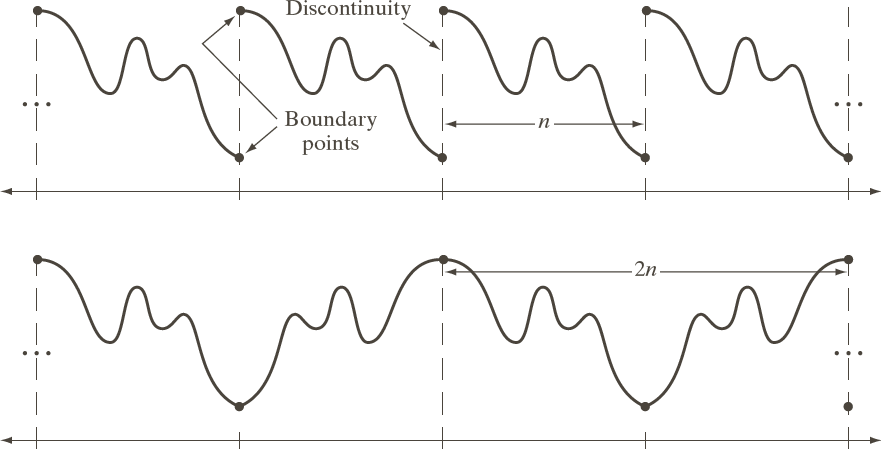
Why are we using the DCT instead of the DFT? First, with the DCT, the coefficients are real numbers. Second, with the DCT, there is no discontinuity at period boudaries. The figure below shows, in the top row, how the DFT considers its input to be periodic and, in the bottom row, how the DCT does this. The DCT has no implicit discontinuities, which means that fewer terms in the series are needed to achieve the same accuracy than would be needed if a discontinuity did exist. See the Wikipedia article for more details.
 [ Gonzales & Woods figure 8.25 ]
The result from Step 4 is a matrix of coefficients, $F(u,v)$, for each of the Y, Cr, and Cb channels. The low-frequency coefficients are in the upper-left corner of the matrix, and with frequency increasing with distance from that corner (just as with the Fourier Transform).
The $F_\textrm{Y}(x,y)$ matrix is $8 \times 8$, while the $F_\textrm{Cr}(x,y)$ and $F_\textrm{Cb}(x,y)$ matrices might be $8 \times 8$ or $4 \times 4$.
The goal in this step is to make many coefficients zero, so that we can use run-length encoding (RLE) on the zeros.
Since the eye is more sensitive to low frequencies, we can lose more resolution in the high frequencies.
In the context of JPEGs, quantization is the act of removing some of the least-significant bits of a DCT coefficient.
Here are two examples of quantization: $$\begin{array}{rcl} 01100011 & { \div \; 4 \atop \longrightarrow } & 011000 \\ \\ 01100011 & { \div \; 16 \atop \longrightarrow } & 0110 \\ \end{array}$$
We don't have to quantize by powers of two, as long as we round the answer: $$\begin{array}{rcl} 01100011 & { \div \; 19 \atop \longrightarrow } & 0101 \end{array}$$
Above, $99 \; \div \; 19 = 5.21$ which, rounded, is $5$.
JPEG uses quantization tables (QT) that provide the divisor of each coefficient in the $8 \times 8$ block of DCT coefficients. These quantization tables vary with JPEG implementations and are stored as part of the image data (unless one of a number of predefined QTs is used).
For example, the Canon EOS 10D camera uses different quantization table for the luminance (Y) channel with its "normal" and "fine" resolutions: $$\begin{array}{ccc} \textrm{Luminance QT: fine} & & \textrm{Luminance QT: normal} \\ \\ \begin{array}{cccccccc} 1 & 1 & 1 & 1 & 1 & 2 & 3 & 3 \\ 1 & 1 & 1 & 1 & 1 & 3 & 3 & 3 \\ 1 & 1 & 1 & 1 & 2 & 3 & 3 & 3 \\ 1 & 1 & 1 & 1 & 3 & 4 & 4 & 3 \\ 1 & 1 & 2 & 3 & 3 & 5 & 5 & 4 \\ 1 & 2 & 3 & 3 & 4 & 5 & 6 & 5 \\ 2 & 3 & 4 & 4 & 5 & 6 & 6 & 5 \\ 4 & 5 & 5 & 5 & 6 & 5 & 5 & 5 \\ \end{array} & \qquad & \begin{array}{cccccccc} 3 & 2 & 2 & 3 & 5 & 8 & 10 & 12 \\ 2 & 2 & 3 & 4 & 5 & 11 & 11 & 13 \\ 3 & 2 & 3 & 5 & 8 & 11 & 13 & 11 \\ 3 & 3 & 4 & 6 & 10 & 17 & 15 & 12 \\ 3 & 4 & 7 & 11 & 13 & 21 & 20 & 15 \\ 5 & 7 & 10 & 12 & 15 & 20 & 21 & 17 \\ 9 & 12 & 15 & 17 & 20 & 23 & 23 & 19 \\ 14 & 17 & 18 & 19 & 21 & 19 & 20 & 19 \\ \end{array} \\ \end{array}$$
Notice how the 'fine' QT uses much smaller divisors to quantize the DCT coefficients; this means that less information will be lost by quantizing in 'fine' than in 'normal'.
Notice also that the divisors generally get larger with increasing frequency (i.e. down and to the right). This is because the eye is less sensitive to errors in high-frequency components than in low-frequency components, so we can afford to lose more information (by using greater divisors) in the high-frequency components.
There are separate quantization tables for the chroma channels. Since the eye is more sensitive to luminance, the chroma QTs usually have larger coefficients.
Given a quantization table, $QT(u,v)$, and a block of DCT coefficients, $F(u,v)$, the quantized coefficients are $$\widehat{F}(u,v) = \textrm{round}(\ F(u,v) \; \div \; QT(u,v)\ ).$$
This will result in many entries equal to zero, which will be compressed with run-length encoding in Step 6.
Here's an example of the quantization step (from Robski Photography):

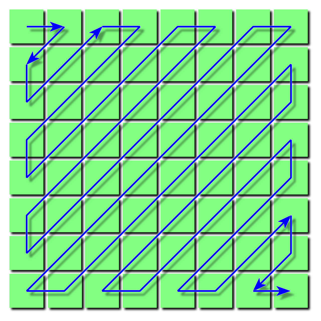
Given the $8 \times 8$ table of quantized coefficients, $\widehat{F}(u,v)$, we now linearize the 64 elements by enumerating them in a zig-zag pattern, as shown below:
 [ Alex Khristov on Wikipedia ]
Recall that the low-ferquency components are in the upper-left. This zig-zag pattern collects the component in approximate order of increasing frequency.
Since we expect that many of the high-frequency component will be zero after quantization, there should be a lot of zeroes at the end of this sequence of 64 linearized coefficients. For example, the "Result" matrix shown above is linearized as $$20, 5, -3, -1, -2, -3, 1, 1, -1, -1 0, 0, 1, 2, 3, -2, 1, 1, 0, 0, 0, 0, 0, 0, 1, 1, 0, 1, 0, 0, 0, 0, 0, 0, 0, 0, 0, 0, 0\ldots$$
The result of linearization is
The DC and AC components from Step 6 are treated differently.
For the DC components:
For Y, Cr, and Cb separately:
For the AC components:
For each $8 \times 8$ block separately:
For Y, Cr, and Cb separately:
Here's an example of encoding, then decoding a small image. This is from Gonzales & Woods Chapter 8.
Original image
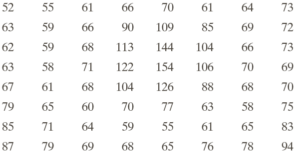
After subtracting 128
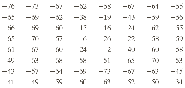
After the DCT
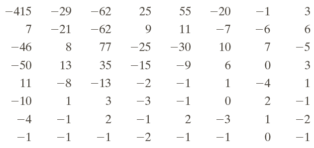
After quantizing
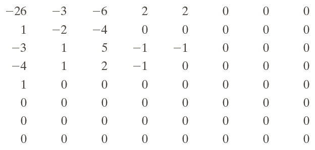
After zig-zag linearization

After RLE and Huffman

Encoded image

After RLE and Huffman
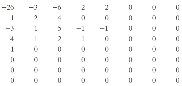
After de-quantization
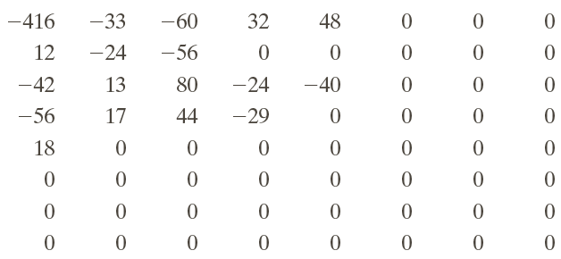
After inverse DCT
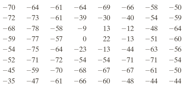
After adding 128
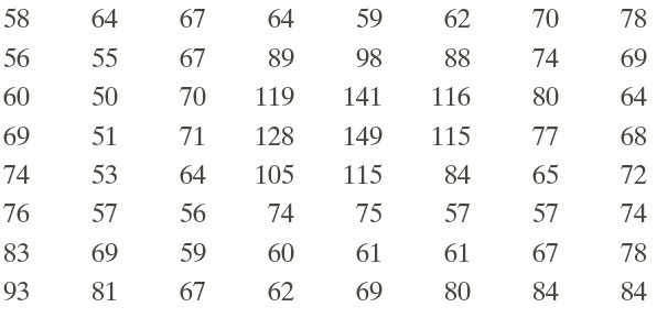
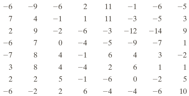
In this case, the loss occured with the quantization / de-quantization steps.
In other cases, there may also be error from the optional subsampling of chroma blocks.
But error is mainly controlled by the quantization table that is chosen.