Canny Edge Detection
Edge detection is used to segment objects in the image. Edge
detection can simplify the process by removing all of the
non-edge pixels, and can sometimes produce more accurate object
segmentation.
We could detect edges by convolving the image with a
first-order finite difference (i.e. edge-detection) filter, then
simple thresholding the resulting values to identify the pixels
on "strong" edges (i.e. those in which there's a fast change in
intensity). But, as we saw in the previous notes, simple
thresholding does not usually do a good job.
The Canny edge detection algorithm, developed by and named
after computer scientist John Canny, does a better job. It
performs five steps:
- Smoothing: Smooth the image to reduce the noise,
which might otherwise result in spurious edges.
- Gradient computation: Compute the gradient
magnitude and direction at each pixel. The magnitude is
larger on strong edges, and the direction is perpendicular
to the edge.
- Suppression of non-maxima: Keep only the pixels with
gradient magnitude that is a local maximum in the
direction perpendicular to the edge. If a pixel does not
have a locally-maximal gradient magnitude, then there's an
adjacent pixel with a larger magnitude which would be a
better representative of this edge.
- Thresholding: Remove pixels with gradient
magnitudes below a certain value, accept those above another
value, and marks as "potential edge pixel" those that are
between.
- Edge extension: Extend the edges consisting of
accepted edge pixels into adjacent potential edge pixels;
the adjacency lends more weight to the likelihood that the
potential edge pixel is a real edge pixel.
1. Smoothing
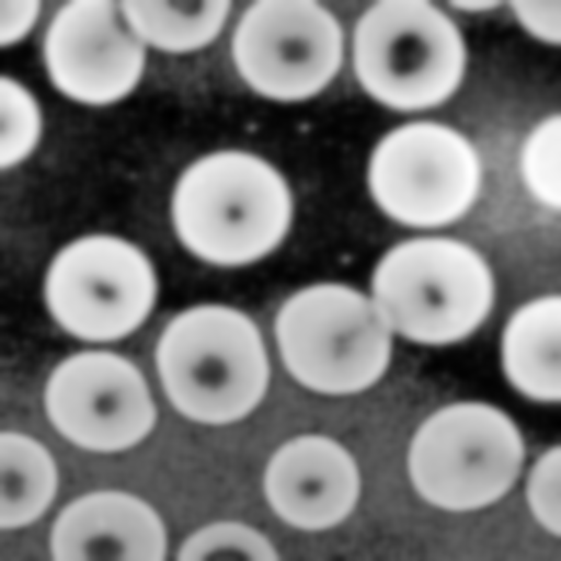
We'll use this as our original image. The objective is to
segment the cells in order to count them:

Some of the images below are generated from
the demonstration
by the Biomedical Imaging Group at the EPFL in Switzerland.
They also have many other
image processing demonstrations. Note that their
demonstration does not show step 4, below.
We first smooth the image with a Gaussian in order to remove
noise, so that noise will not been mistaken for edges by the
algorithm. We can choose the standard deviation of the
Gaussian: a larger standard deviation will result in a smoother
image, but some detail might get lost.
Here's the smoothed image using a Gaussian with standard
deviation of 4 pixels:

2. Gradient Computation
We next convolve two smoothed central difference filters with
the image: one filter computes the gradient, $G_x$, in the $x$
direction, while the other computes the gradient, $G_y$, in the
$y$ direction.
$$F_x = \left[ \begin{array}{rrr} -1 & 0 & 1 \\ -2 & 0 & 2 \\ -1 & 0 & 1 \end{array} \right]
\qquad
F_y = \left[ \begin{array}{rrr} 1 & 2 & 1 \\ 0 & 0 & 0 \\ -1 & -2 & -1 \end{array} \right]$$
Then the gradient at a pixel is $G = (G_x,G_y)$ with magnitude $\sqrt{
G_x^2 + G_y^2 }$ and direction $\arctan( {G_y \over G_x} )$.
Note that the directions span the range of $[-{\pi \over
2},{\pi \over 2}]$ and the gradient $(G_x,G_y)$ has the same
computed "direction" as the gradient $(-G_x,-G_y)$. This is
good, as an edge with a gradient up-and-right will be
considered to have the same direction as an edge with a
gradient down-and-left.
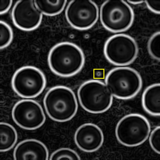
Here's the smoothed image with intensities proportional to
gradient magnitude:

In the next step (#3) we'll be looking at adjacent pixels in
the direction of the gradient. To make the lookup of adjacent
pixels easier, we'll discretize the gradient
directions, $\arctan( {G_y \over G_x} )$, into vertical,
horizontal, and two diagonal directions.
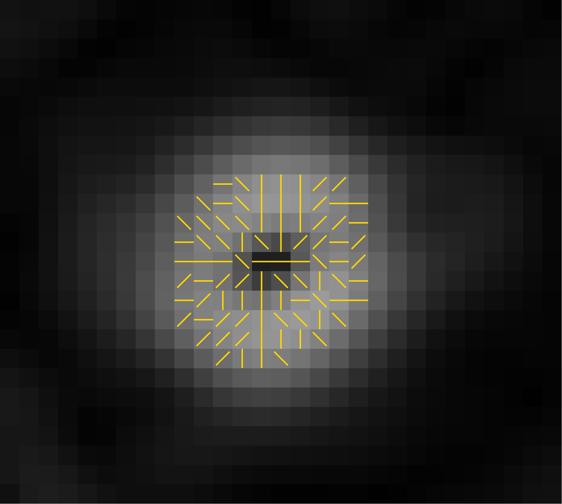
Below is a zoomed in part of the gradient magnitude image
from the yellow box in the image above. This shows, for
selected pixels, the discretized gradient directions.

3. Suppression of Non-maxima
When we threshold the gradient magnitude in the next step (#4),
we want a single line of pixels to be detected for each edge.
However, the smoothing operation (#1) will have caused edges to
become several pixels wide, and thresholding by
gradient magnitude would produce a thick line of pixels
covering the whole width of the smoothed edge.
So we will pick only the pixel that is a local maximum in
the direction of the gradient. This is the direction
perpendicular to the edge, so following this direction takes
us across the width of the edge.
At each pixel, we look at the two adjacent pixels in the
direction of the gradient. If either of those has a larger
gradient magnitude, we suppress the pixel.
Here are the locally maximal pixels from the image above, shown with red dots:

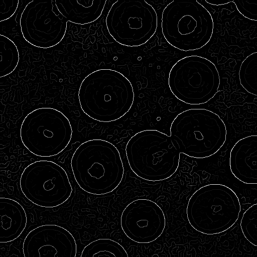
And here's the image after we have suppressed (i.e. set to black)
the pixels that are not locally maximal in their gradient
direction:

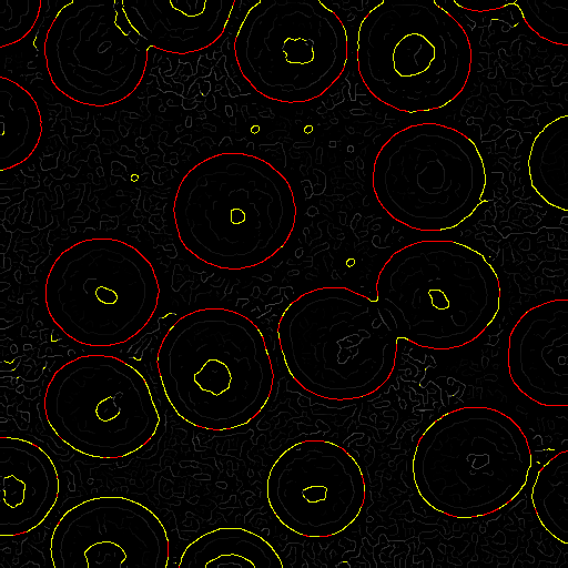
4. Thresholding
We next classify the pixels as "not edge", "potential edge",
and "edge" based on two thresholds, $\tau_1$ and $\tau_2$, with
$\tau_1 \lt \tau_2$:
- "not edge" has gradient magnitude less than $\tau_1$.
- "potential edge" has gradient magnitude between $\tau_1$ and $\tau_2$.
- "edge" has gradient magnitude greater than $\tau_2$.
Here's an example classification with red "edge" pixels and
yellow "potential edge" pixels:

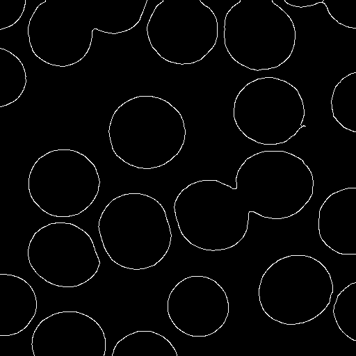
5. Edge extension
Finally, we extend the edge pixels (red above)
into adjacent potential edge pixels (yellow above).
This has the effect of filling gaps in the edges.
To do so, we put all edge pixels into a queue and remove them
one-by-one. Upon removing a pixel from the queue, we look at
its eight adjacent pixels. Any that are potential edge pixels
are changed to edge pixels and are added to the queue.
Once the queue is empty, we discard the remaining potential
edge pixels (which were not attached to any edge pixels) and are
left with a set of edge pixels, as shown below:
Try It Yourself
Step through the
online demonstration
with different standard deviations, different thresholds, and
different images.
up to Schedule & Notes

