The Laplacian finds high-curvature (i.e. high frequency) parts of the image.
The second derivative really emphasizes noise in the original image.
We should reduce image noise before applying the Laplacian if doing analysis to find edges. We don't want to find spurious edges from the noise.
Solution: First use a Gaussian smoothing filter to reduce the noise: $$\begin{array}{rll} & (I ∗ G) ∗ ∇² & \textrm{for Gaussian } G \textrm{ and Laplacian } ∇² \\ = & I ∗ (G ∗ ∇²) & \\ = & I ∗ (∇² \; G) & \textrm{where } ∇²G \textrm{ is the Laplacian of a (continuous) Gaussian} \\ \end{array}$$
where $$\begin{array}{rl} (G ∗ ∇²) = & {1 \over 16} \left[\begin{array}{ccc} 1 & 2 & 1 \\ 2 & 4 & 2 \\ 1 & 2 & 1 \\ \end{array}\right] ∗ \left[\begin{array}{ccc} 1 & 1 & 1 \\ 1 & -8 & 1 \\ 1 & 1 & 1 \\ \end{array}\right] \\ \\ = & {1 \over 16} \left[\begin{array}{ccccc} 1 & 3 & 4 & 3 & 1 \\ 3 & 0 & -6 & 0 & 3 \\ 4 & -6 &-20 & -6 & 4 \\ 3 & 0 & -6 & 0 & 3 \\ 1 & 3 & 4 & 3 & 1 \\ \end{array}\right] \\ \end{array}$$
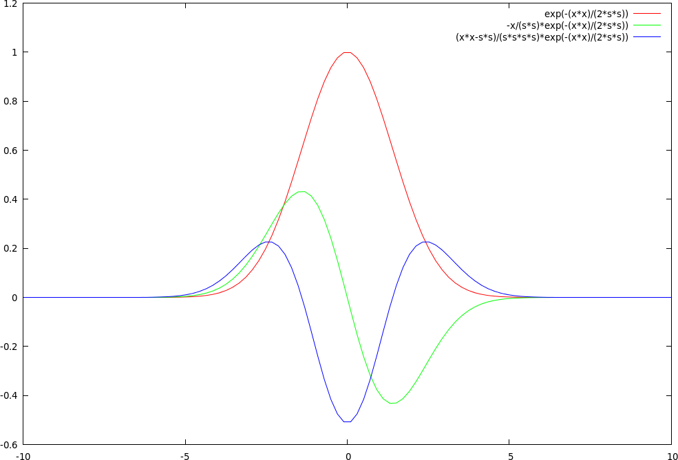
In 1D without the normalizing factor, the Gaussian and its derivatives are: $$\begin{array}{lll} G(x) & = e^{-{x^2 \over 2 \sigma^2}} \\ G_x(x) & = -{x \over \sigma^2} e^{-{x^2 \over 2 \sigma^2}} & \textrm{first partial derivative with respect to } x \\ G_{xx}(x) & = {x^2-\sigma^2 \over \sigma^4} e^{-{x^2 \over 2 \sigma^2}} & \textrm{second partial with respect to } x = \textrm{ Laplacian of Gaussian (LoG)} \\ \end{array}$$
Below are the Gaussian (one peak in red), its first derivative (two peaks in green), and its second derivative (i.e. the Laplacian of the Gaussian) (three peaks in blue):
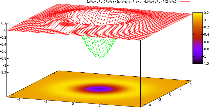
In 2D, the Laplacian of the Gaussian looks like the image below. $$\begin{array}{rl} ∇²G = & G_{xx} + G_{yy} \\ = & {x^2+y^2-2\sigma^2 \over \sigma^4}e^{-{x^2+y^2 \over 2 \sigma^2}} \\ \end{array}$$
The Difference of Gaussians (DoG)
The LoG is not separable, so can be expensive for large $\sigma$.
We can approximate $\nabla^2 G$ with a "difference of Gaussians": $G_1 - G_2$
$I ∗ (G_1 - G_2) = I ∗ G_1 - I ∗ G_2$
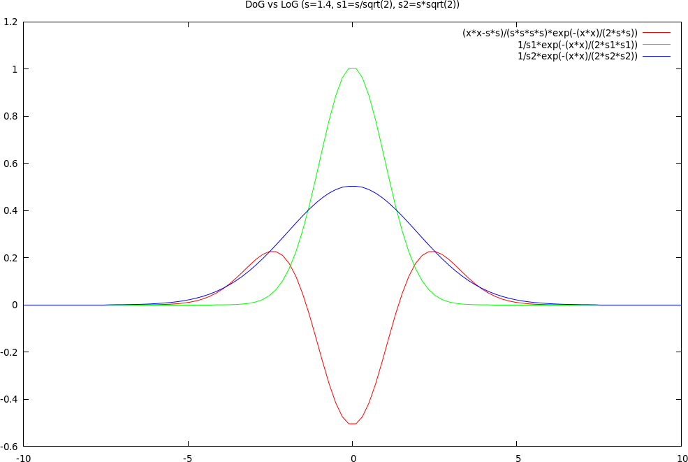
Here are a Gaussian with small sigma (tall peak in green), a Gaussian with larger sigma (shorter peak in blue), and their difference (three peaks in red):
And below we compare the Difference of Gaussians (slightly higher three peaks in red) with the Laplacian of the Gaussian (slighter lower three peaks in pink):
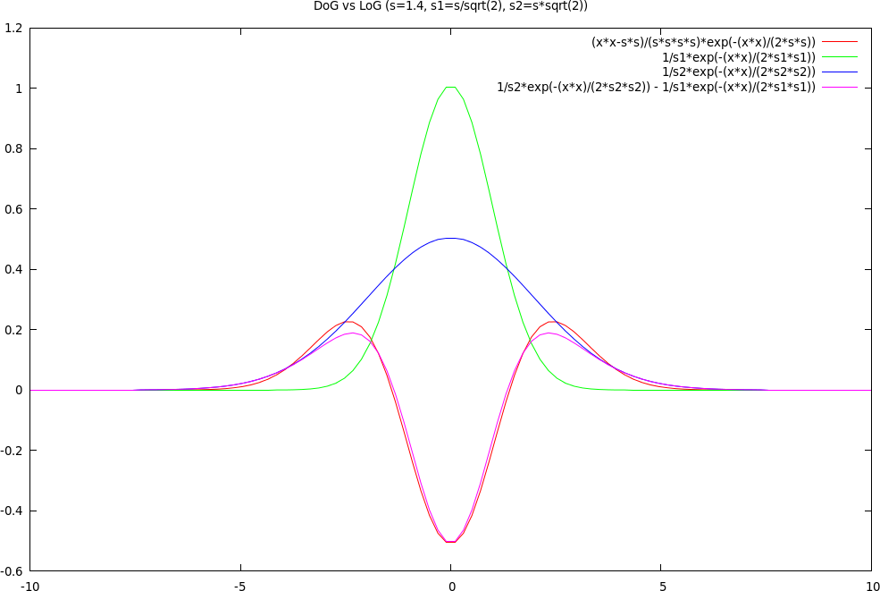
The DoG does approximately what the LoG does but, since Gaussians are separable, this DoG is much cheaper to compute with than the LoG.
Some Intuition
A Gaussian, G, smooths the image, removing (i.e. filtering out) high-frequency noise. The larger the $\sigma$ of G, the more smoothing and the lower the maximum frequency, $f$, above which everthing gets attenuated.
$I * G_1$ contains the spatial frequencies below some threshold, $f_1$, while $I * G_2$ contains the spatial frequencies below another threshold, $f_2$. If $\sigma_1 < \sigma_2$ then $f_1 > f_2$ ... not the other way around. In the figure above, $\sigma_1$ would be that of the tall green Gaussian, while $\sigma_2$ would be that of the shorter blue Gaussian.
Thus $I * G_1 - I * G_2$ contains frequencies below $f_1$, minus those frequencies below $f_2$, leaving untouched the frequencies between $f_1$ and $f_2$, which correspond to image edges of a certain size.