First Derivative in 1D [3.6.1]
The first derivative of $f(x)$ is $${d \over dx} f(x) = \lim_{dx \rightarrow 0} {f(x+dx) - f(x) \over dx}$$
Its discrete approximation (with $dx = 1$) is $$\begin{array}{rl} {d \over dx} f(x) \approx & {f(x+1) - f(x) \over 1} \\ \approx & {f(x+1) - f(x-1) \over 2} \qquad \textrm{to centre it on } x \\ \end{array}$$
The corresponding discrete kernel is $$\begin{array}{|r|c|c|c|} \hline \textrm{weight} & -0.5 & 0 & 0.5 \\ \hline \textrm{index} & -1 & 0 & +1 \\ \hline \end{array}$$
This must be rotated by 180$^o$ if it is to be a convolution filter.
First Derivative in 2D
Here is one possible first derivative filter in 2D: $$\begin{array}{|c|c|c|} \hline -1 & 0 & 1 \\ \hline -2 & 0 & 2 \\ \hline -1 & 0 & 1 \\ \hline \end{array}$$
This must be rotated by 180$^o$ if it is to be a convolution filter.
- What does this compute?
solutionThe first derivative in the horizontal direction
- Why are there three rows?
solutionSo as to take a weighted average of the three first derivatives in those rows.
Second Derivative in 1D
The second derivative of $f(x)$ is $$\begin{array}{rl} \large {d \over dx} ( {d \over dx} f(x) ) = & \lim_{dx \rightarrow 0} \large { {d \over dx} f(x+dx) - {d \over dx} f(x) \over dx } \\ = & \lim_{dx \rightarrow 0} \large { (f(x+dx+dx) - f(x+dx)) - (f(x+dx) - f(x)) \over {dx}^2 } \\ = & \lim_{dx \rightarrow 0} \large { f(x+2 dx) - 2 f(x+dx) + f(x) \over {dx}^2 } \\ = & \lim_{dx \rightarrow 0} \large { f(x+dx) - 2 f(x) + f(x-dx) \over {dx}^2 } \quad \textrm{to centre it on } x \\ \end{array}$$
Its discrete approximation (with $dx = 1$) is $${d^2 \over {dx}^2} f(x) \approx f(x+1) - 2f(x) + f(x-1)$$
The corresponding discrete kernel is $$\begin{array}{|r|c|c|c|} \hline \textrm{weight} & 1 & -2 & 1 \\ \hline \textrm{index} & -1 & 0 & +1 \\ \hline \end{array}$$
This is the same as if it were rotated by 180$^o$, so can be used as-is for convolutions.
Sharpening
We can sharpen an image by subtracting some amount, say 10%, of the second derivative at each point in the signal: $$\begin{array}{cccl} 0.0 & 1.0 & 0.0 & (i =\textrm{ filter to get original signal}) \\ 0.1 & -0.2 & 0.1 & (d =\textrm{ filter to get 10% of second derivative}) \\ \hline -0.1 & 1.2 & -0.1 & (i-d =\textrm{ difference of filters}) \\ \end{array}$$
See the applet to experiment with this.
This works because convolution is distributive: $$\begin{array}{rl} & f(x) - (d∗f)(x) \\ = & (i∗f)(x) - (d∗f)(x) \\ = & ((i-d)∗f)(x) \\ \end{array}$$
This is often written without the parameter: $$\begin{array}{rl} & f - d∗f \\ = & i∗f - d∗f \\ = & (i-d)∗f \\ \end{array}$$
The Laplacian
The "Laplace operator" or "Laplacian" ∇² is the divergence of the gradient of a field.
For field $f(x), ∇²f(x) = δ²f/δx²$
For field $f(x,y,z), ∇²f(x) = δ²f/δx² + δ²f/δy² + δ²f/δz²$
$∇²f(x)$ is the average difference between ($f$ in the immediate (spherical) neighbourhood of $x$) and $f$ at $x$ itself, divided by the distance from $x$ to its neighbourhood. In other words, this is the average rate of change over directions passing through $x$.
The "discrete Laplacian filter" is the discrete approximation of $∇²f$. $$\begin{array}{rl} ∇²f(x) \approx & f(x+1) - 2f(x) + f(x-1) \\ \\ = & \left[ \begin{array}{ccc} 1 & -2 & 1 \end{array}\right] \quad \textrm{as a filter} \\ \end{array}$$
In 2D this is $$\begin{array}{rl} ∇²f(x,y) \approx & (f(x+1,y) - 2f(x,y) + f(x-1,y)) + (f(x,y+1) - 2f(x,y) + f(x,y-1)) \\ \\ = & \left[ \begin{array}{ccc} 0 & 1 & 0 \\ 1 & -4 & 1 \\ 0 & 1 & 0 \\ \end{array} \right] \quad\textrm{as a filter} \\ \end{array}$$
Note how this is the average difference (in four directions) of the adjacent value and the centre value.
Problem: This only detects the second derivative in the $x$ and $y$ directions.
A more symmetrical filter is $$\left[\begin{array}{ccc} 1 & 1 & 1 \\ 1 & -8 & 1 \\ 1 & 1 & 1 \\ \end{array}\right]$$
- What does this detect?
solutionAverage curvature in all directions.
- Is it directional?
solutionThere's a slight bias toward the horizontal, vertical, and diagonal directions.
Sharpening with the Laplacian
To sharpen an image $p(x,y)$:
- Convolve $p(x,y)$ with a Laplacian to get the "Laplacian image", $L(x,y)$.
- Normalize Laplacian image so all values are in [-1,+1].
- For each pixel at $(x,y)$:
$p'(x,y) = p(x,y) - k * L(x,y)$
(Choose k to affect how much sharpening is added.)
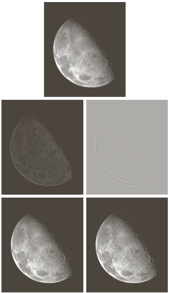
Below is a figure [Gonzales & Woods Fig 3.38] showing
- top: original image
- middle left: Laplacian of image
- middle right: Laplacian of image scaled so that zero is grey, white is positive, black is negative
- bottom left: image sharpened by adding horizontal/vertical Laplacian
- bottom right: image sharpened by adding horizontal/vertical/diagonal Laplacian
