$I$ = image, $H$ = filter (which can also be thought of as an image).
Definition of convolution:
$$(I ∗ H)(x,y) = \sum_i \sum_j ( I(x-i,y-j) H(i,j) )$$
Convolution is commutative
Proof that $H1 ∗ H2 = H2 ∗ H1$:
First, however, note that
$$\begin{array}{ccccc}
\sum_{i=a}^b f(i) &=& \sum_{i=a-c}^{b-c} f(i+c) &=& \sum_{i=-(a-c)}^{-(b-c)} f(-i+c) \\
[a \ldots b] && [a-c+c \ldots b-c+c] && [-(-(a-c))+c \ldots -(-(b-c))+c] \\
\end{array}$$
and, if $a = -\infty$ and $b = +\infty$, limits of summation do not change.
Proof in 1D:
$$\begin{array}{rl}
(H1 ∗ H2)(x) = & \sum_i H1(x-i) \; H2(i) \\
= & \sum_i H1(x-(x-i))) \; H2(x-i) \qquad \textrm{substitute } i \rightarrow x-i = -(i-x) \textrm{ in the sum} \\
= & \sum_i H1(i) \; H2(x-i) \\
= & \sum_i H2(x-i) \; H1(i) \\
= & (H2 ∗ H1)(x) \\
\end{array}$$
Run the "convolve" code to experiment with this.
Convolution is associative
Proof in 1D that $I ∗ (H1 ∗ H2) = (I ∗ H1) ∗ H2$:
$$\begin{array}{rl}
(I ∗ (H1 ∗ H2))(x) = & \sum_i ( I(x-i) (H1 ∗ H2)(i) ) \\
= & \sum_i ( I(x-i) \sum_j ( H1(i-j) H2(j) ) ) \\
= & \sum_j ( ( \sum_i I(x-i) H1(i-j) ) H2(j) ) \\
= & \sum_j ( ( \sum_i I(x-(i+j)) H1((i+j)-j) ) H2(j) ) \qquad \textrm{substitute } i \rightarrow i+j \textrm{ in the sum} \\
= & \sum_j ( ( \sum_i I((x-j)-i) H1(i) ) H2(j) ) \\
= & \sum_j ( (I ∗ H1)(x-j) H2(j) ) \\
= & ((I ∗ H1) ∗ H2)(x) \\
\end{array}$$
Covolution has an identity element
Convolution is linear
For a scalar $a$:
$$(a I) ∗ H = a (I ∗ H)$$
and
$$(I1 + I2) ∗ H = (I1 ∗ H) + (I2 ∗ H)$$
(no proof)
Convolution is shift invariant
A shift of 2D image $I$ by $(a,b)$ is denoted $S_{ab}(I)$ and is defined as
$$S_{ab} (I)(x,y) = I(x-a,y-b)$$
An operation (such as convolution) is "shift invariant" if
the position at which the operation is applied has no
effect on the transform. In other words:
$$S_{ab} (I) ∗ H = S_{ab} (I ∗ H)$$
Differentiation is easy with convolution
$${d \over dx} (H1 \; ∗ \; H2) = {d \over dx}(H1) \; ∗ \; H2$$
Theorem: The only shift-invariant, linear operators on
images are convolutions.
"LTI" = "Linear time invariant" or "Linear translation invariant"
Averaging in 1D
A box filter has equal weights symmetric about the
weight's origin, like the averaging filter we saw before.
A Gaussian filter has a Gaussian centred at the filter's
origin:
$$G(x) = {1 \over \sigma \; \sqrt{2 \pi}} \; e^{ {-1 \over 2} \; \left( { x - \mu \over \sigma } \right)^2 }$$
A discrete version of the Gaussian has a finite width
and approximates the value of the continuous Gaussian at discrete
points. In the range [-2,+2], the weights are:
0.06136 0.24477 0.38774 0.24477 0.06136 (from http://dev.theomader.com/gaussian-kernel-calculator/)
See the applet to experiment with this.
Convolving a box filter with itself multiple times results in
an approximate Gaussian (and is a Gaussian in the limit).
This applies to *any* filter, not just the box!
Run the "convolve" code to experiment with this.
Averaging in 2D
The box and Gaussian filters are similar in 2D. The middle
image below is the result of a 15x15 box filter applied to a
sky image on the left:
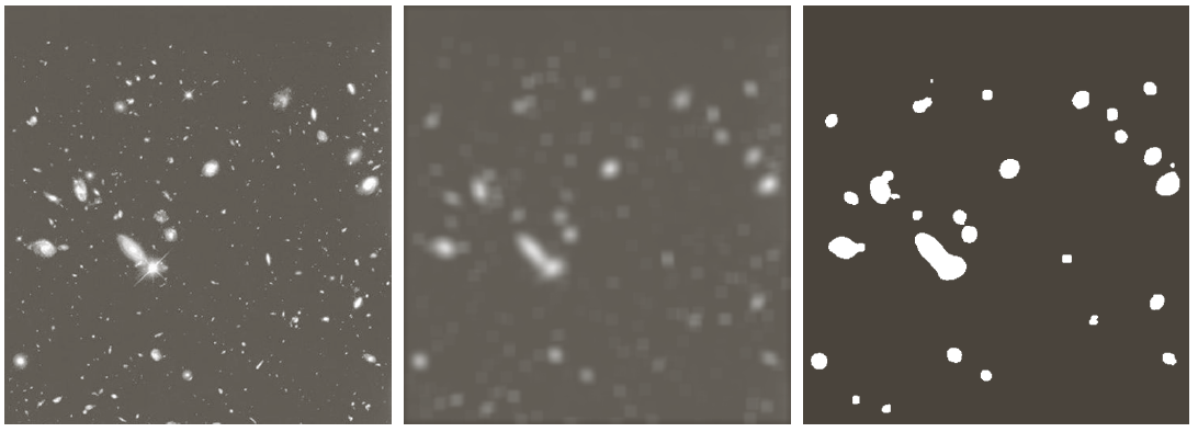 [ Gonzales & Woods Fig 3.34 ]
The right image above is a thresholding of the middle image.
Standard Form of Convolution
The standard form is
$$(w ∗ p)(x,y) = { \sum_i \sum_i w(i,j) \; p(x-i,y-j) \over \sum_i \sum_j w(i,j) }$$
The denominator ensures that the sum of the weights, $w(i,j)$, is normalized to 1, as
$${\sum_i \sum_j w(i,j) \over \sum_i \sum_j w(i,j)} = 1$$