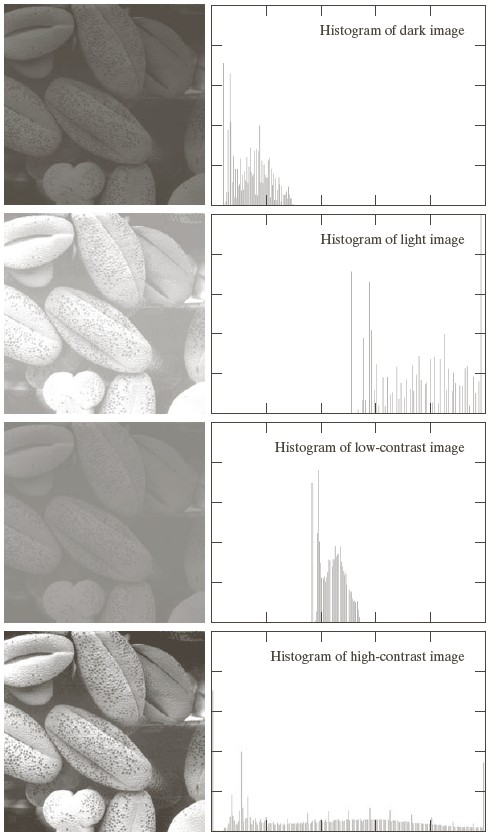
 [ Gonzales & Woods Fig 3.16 ]
A histogram, $h(i)$, stores the number of pixels in image with value $i$.
You can characterize histograms for dark, light, low constrast, high contrast images, as shown below. In the histograms below, the horizontal axis is the pixel value, while the vertical axis is the number of pixels at that value.
 [ Gonzales & Woods Fig 3.16 ]
"Contrast stretching" map some range of pixels to a broader range, while compressing the other ranges. This can be used to enhance image contrast.
The image below shows the mapping, $s = T(r)$, in the upper-left corner. The axes are in the range [0,L-1] instead of our usual [0,1], since the book uses $L$ as the number of intensity levels (e.g. L=256).
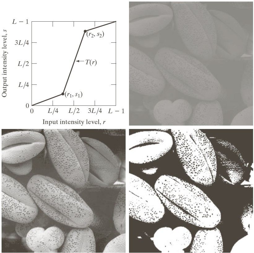
 [ Gonzales & Woods Gig 3.10 ]
Histogram equalization is, in a sense, automatic contrast stretching.
We want to "flatten" the histogram so that all pixel intensities occur in the same number. For 256 intensities and N total pixels, each intensity in [0,255] appears N/256 times.
Here's what happens if we apply histogram equalization to the four images above:
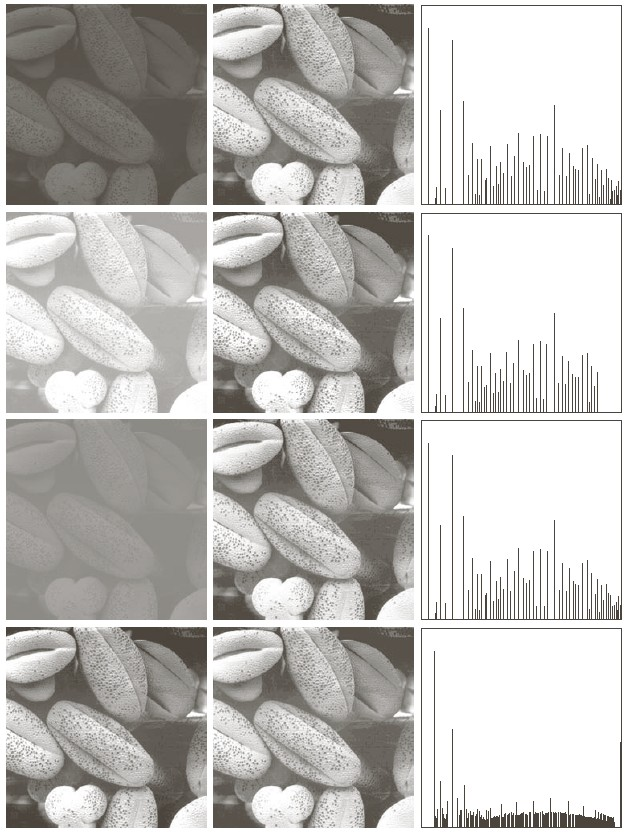
We want to map intensity $r$ in image $R$ to intensity $s$ in image $S$ so that the intensities in $S$ have a flat histogram.
That mapping is $s = T(r)$. How do we determine $T$?
Suppose there are $N_r$ pixels in $R$ of intensity at most $r$. In other words,
$N_r = \sum_{i=0}^{r} h_R(i)$
($h_R(i)$ is the number of pixels at intensity $i$ in image $R$.)
Ideally, in a flat distribution, those $N_r$ pixels from the left side of the histogram of $R$ (they're on the left since they're between 0 and $r$) are mapped to the left side of the histogram of $S$. They thus have intensities between 0 and some intensity, $s$, such that
$\begin{array}{rl} N_r = & \textrm{number of pixels with intensity at most } s \\ = & (s+1) N / 256 \\ \end{array}$
since each of the $s+1$ intensities in $[0,s]$ has $N / 256$ pixels of that intensity in image $S$, which has a flat histogram).
Then
$N (s+1) / 256 = \sum_{i=0}^{r} h_R(i)$
and
$\begin{array}{rl} s = & ( 256 / N \; \sum_{i=0}^{r} h_R(i) ) - 1 \\ = & T(r) \\ \end{array}$
To perform histogram equalization, compute $T(r)$ for each value of $r$ and store in a look-up table. Then go through all the pixels in $R$ and replace each pixel's instensity, $r$, with $T(r)$.
Building the lookup table can be done in a loop in time linear in the number of pixels and intensity values.
$s = T(r)$ is almost never an integer; it's a fractional number that gets truncated or rounded.
This causes gaps in the histogram and an uneven spread of values.
[ CODE DEMO OF HISTOGRAMS AND THE MAPPING FUNCTION ]
Looking at the case of continuous intensity values can give you some insight into what's going on here.
Let $d_i$ be an infinitesimally small range of intensities (instead of, for example, the range [128,129) ).
Let $p_r(i)$ be the probability density that a randomly chosen pixel in $R$ has intensity $i$.
"Probability density" means "probability per some measure" where the measure is a range of intensities in this case.
Then $p_r(i) \; d_i$ is the probability (not "probability density") that a randomly chosen pixel in R has intensity i. This is just $h_R(i) / N$, since that's the fraction of pixels of intensity $i$.
Then
$\begin{array}{rl} \int_{i=0}^{r} p_r(i) \; d_i = & \int_{j=0}^{s} p_s(j) \; d_j \\ = & s / 256 \qquad \textrm{since } p_s(j) \textrm{ is constant and equal to } 1/256 \\ \end{array}$
So
$s = T(r) = 256 \int_{i=0}^{r} p_r(i) \; d_i$
Instead of applying the histogram equalization over the whole image, apply it to small areas, separately.
In each small area, use the area to compute the transformation, $s = T(r)$, but use that transformation on only the centre pixel of the area [fig 3.26]
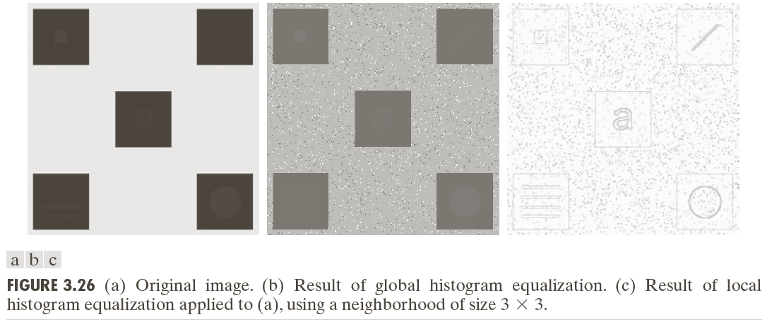 [ Gonzales & Woods ]
Problem: This can enhance noise in smooth regions.