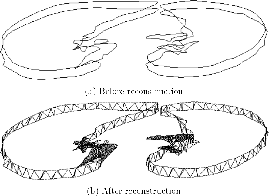
Consider the contour joining problem, in which we have two parallel planes with a polygonal contour in each plane, and want to join the countours with a triangulation.
This data can come from medical imaging, where the parallel planes are "slices" taken by CT imaging and the polygonal contour is the outline of a bone or organ.
Here are two parallel slices from a lung CT and their triangulation.

|
| [ Barequet and Sharir, "Piecewise-Linear Interpolation between Polygonal Slices", Symposium on Computational Geometry, 1994 ] |
|---|
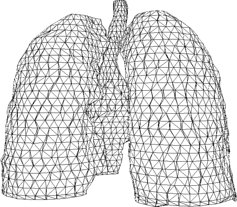
By triangulating each adjacent pair of slices from the CT, we can build up a 3D model of the bone or organ.

|
| [ Barequet and Sharir, "Piecewise-Linear Interpolation between Polygonal Slices", Symposium on Computational Geometry, 1994 ] |
|---|
Here's a closeup of parts of two contours, with a triangulation between them:
The vertices on top and bottom are indexed. Edges between the top and bottom can be described by pairs of indices, such as $(1,1)$ for the leftmost edge and $(8,5)$ for the rightmost edge.
This triangulation can be thought of as a path through a rectangular graph, where each node is labelled as $(i,j)$ for $i$ a vertex in the bottom contour and $j$ a vertex in the top contour:
Each node visited on the path corresponds to an triangle edge in the triangulation.
Each edge traversed on the path corresponds to a triangle in the triangulation.
The minimum area contour problem is to join two polygonal contours, such as described above, with a minimum area triangulation. Such a triangulation usually results in a "natural looking" surface between the contours.
Since each edge of the rectangular graph corresponds to a triangle, we can weight each edge with that triangle's area.
Then the problem is to find the minimum-weight path between the upper-left corner and the lower-right corner. (It's a bit more complicated, as we have to ensure that we pick a "good" initial pair of top and bottom vertices. And the last pair of vertices has to be the same as the first pair of vertices if the contour is to be closed.)
We could do this with Dijkstra's algorithm, but let's try something different ...
We'll define the problem recursively: Let $\ma(i,j)$ be the area of the minimum-area triangulation that starts with edge $(1,1)$ and ends with edge $(i,j)$.
Since we can arrive at $(i,j)$ from only two other vertices in the graph (i.e. the vertices above $(i,j)$ and left of $(i,j)$), we get this recurrence relation: $$\ma(i,j) = \begin{array}[t]{rl} \min( & \ma(i-1,j) + \a( (i-1,j), (i,j) ), \\ & \ma(i,j-1) + \a( (i,j-1),(i,j) )\ \ \ ) \end{array}$$
where $\a( (i,j), (k,\ell) )$ is the area of the triangle defined by edges $(i,j)$ and $(k,\ell)$.
We should also define $\ma(0,j) = \ma(i,0) = \infty$ to ensure that we don't try to make a triangle to the left of the leftmost edge or above the top edge of the rectangular graph.
Solving the recurrence relation blindly would cost time exponential in the number of contour vertices. That's because the problem size is the number of edges to be traversed, and evaluation of one level of the recurrence requires solving two problems, each of size one less than the original size: $$T(i,j) = 1 + T(i-1,j) + T(i,j-1)$$
So the number of evaluations required for a path of length $i+j$ is two times the number of evaluations required for a path of length $i+j-1$. This is $\O( 2^{i+j} )$ which is, essentially, the number of different paths between $(1,1)$ and $(i,j)$.
We can exploit the following observation to solve this recurrence relation more efficiently:
The same subproblem is evaluated many times in the recurrence relation so, instead of evaluting it many times, we should evaluate it once and store the result, so that future evaluations take constant time.
For example, in evaluating $\ma(3,3)$, there are six evaluations of the smaller subproblem of evaluating $\ma(1,1)$, corresponding to the six recursive visits to $(1,1)$ from $(3,3)$. So we should evaluate $\ma(1,1)$ once and store it.
For the Minimum Area Contour, above, we could build a table of 8 rows and 5 colums and store $\ma(i,j)$ in cell $[i,j]$ of the table.
Another key observation is:
Since larger problems require evaluation of smaller subproblems, evaluate and store the subproblems first.
For example, for the Minimum Area Contour we would first evaluate the "smallest" subproblems of $\ma(1,1), \ma(1,2), \ldots, \ma(1,5)$. We would next evaluate the "not quite smallest" subproblems $\ma(2,1), \ma(2,2), \ldots, \ma(2,5)$. This would repeat until we reached $\ma(8,5)$.
Here's the minArea[] table with arrows showing the order in which evaluations are done:
If things are done in this order, the table always has precomputed results for the subproblems that are next to be evaluated.
For example, upon evaluating $\ma(3,4)$, both subproblems $\ma(2,4)$ (above) and $\ma(3,3)$ (left) have already been evaluated (see the minArea[] table above). So $\ma(3,4)$ takes constant time to evaluate.
Solving the problem in this manner takes $O( m\ n )$ time for $m$ vertices on the one contour and $n$ on the other contour.
The algorithm above simply gave us the area of the minimum area triangulation; it didn't list the triangulation.
We could, while building the table, record in each cell whether the minimum-weight path came from above or from the left. Then from cell $(i,j)$ we could walk backward through the table to find all of the triangles on the minimum-weight path.
To avoid the extra storage required by that approach, we could alternatively determine, at each cell $\ma[i,j]$, which of $\ma[i-1,j] + \a((i-1,j),(i,j))$ and $\ma[i,j-1]+\a((i,j-1),(i,j))$ is lower. We would then walk backward in the direction of lower cost to find all of the triangles on the minimum-weight path.
This method of solving problems in an order such that the required subproblems have already been solved and stored before they are needed is called dynamic programming.
We'll generalize this idea in the next set of notes.